Matrice d'une application linéaire

Sommaire

Application linéaire associée à une matrice

Tu souhaites en savoir plus sur la notion de matrice d’une application linéaire ? Améliore tes connaissances sur cette notion grâce à notre article dédié au chapitre : Définition et démonstration : matrice d’une application linéaire. Prochaine étape : réussis toutes tes interrogations écrites et orales sur la notion !

Et si tu veux franchir un nouveau palier dans ta préparation aux examens prends un cours de soutien scolaire d’algèbre. 🎓

Application linéaire canoniquement associée à une matrice

Définitions

Définition : Application linéaire canoniquement associé à une matrice

Soit $A\in\mathcal{M}_{n,p}(\mathbb{K})$

. L’application linéaire de $\mathbb{K}^p$

dans $\mathbb{K}^n$

dont la matrice dans les bases canoniques respectives de $\mathbb{K}^p$

et $\mathbb{K}^n$

est $A$

est appelée application linéaire canoniquement associée à $A$

Remarque : Matrice d’une application linéaire

Soit $A=(a_{i,j})_{\substack{1\leq i\leq n\\ 1 \leq j \leq p}}\in\mathcal{M}_{n,p}(\mathbb{K})$

. L’application linéaire canoniquement associée à $A$

est :

$f : \begin{array}[t]{ccc} \mathbb{K}^p & \to & \mathbb{K}^n\\ (x_1,\dots,x_p) & \mapsto & \left(\underbrace{\sum\limits_{j=1}^pa_{1,j} x_j}_{y_1},\dots,\underbrace{\sum\limits_{j=1}^pa_{n,j} x_j}_{y_n}\right). \end{array}$

De plus, pour simplifier les notations, on identifie tout vecteur de $\mathbb{K}^p$

(resp. de $\mathbb{K}^n$

) à sa matrice des coordonnées dans la base canonique de $\mathbb{K}^p$

(resp. de $\mathbb{K}^n$

).
On identifie $(x_1,\dots,x_p)\in\mathbb{K}^p$

à $X=\begin{pmatrix} x_1\\\vdots\\x_p\end{pmatrix}\in\mathcal{M}_{p,1}(\mathbb{K})$

, et $(y_1,\dots,y_n)\in\mathbb{K}^n$

à $Y=\begin{pmatrix} y_1\\\vdots\\y_n\end{pmatrix}\in \mathcal{M}_{n,1}(\mathbb{K})$

. Avec cette identification, l’application linéaire canoniquement associée à $A$

se réécrit :

$f : \begin{array}[t]{ccc} \mathcal{M}_{p,1}(\mathbb{K}) & \to & \mathcal{M}_{n,1}(\mathbb{K})\\ X & \mapsto & A X (=Y). \end{array}$

Définition : Noyau et image d’une matrice

Soient $A\in\mathcal{M}_{n,p}(\mathbb{K})$

et $f:\mathbb{K}^p\to\mathbb{K}^n$

l’application linéaire canoniquement associée à $A$

Le noyau de $A$

est le noyau de $f$

(c’est un sous-espace vectoriel de $\mathbb{K}^p$

L’image de $A$

est l’image de $f$

(c’est un sous-espace vectoriel de $\mathbb{K}^n$

Remarques

On note $A=(a_{i,j})_{\substack{1\leq i\leq n\\1\leq j\leq p}}\in\mathcal{M}_{n,p}(\mathbb{K})$

Soit $(x_1,\dots,x_p)\in\mathbb{K}^p$

. On a :

$(x_1,\dots,x_p) \in \mathrm{Ker}(A) \Longleftrightarrow A \begin{pmatrix} x_1\\\vdots\\x_p \end{pmatrix}=\begin{pmatrix} 0\\\vdots\\0 \end{pmatrix} \Longleftrightarrow \left\lbrace \begin{array}{cccccccc} a_{1,1} x_1 &+& \dots &+& a_{1,p} x_p&=&0\phantom{.}\\ \vdots&&&&\vdots&&\vdots\\ a_{n,1} x_1 &+& \dots &+& a_{n,p} x_p&=&0.\\ \end{array}\right.$

Les lignes de $A$

donnent un système d’équations linéaires du noyau de $A$

On note $\mathcal{B}=(e_1,\dots,e_p)$

la base canonique de $\mathbb{K}^p$

.
Pour tout $j\in [[1,p]]$

, en identifiant $\mathbb{K}^p$

à $\mathcal{M}_{p,1}(\mathbb{K})$

, on a $A\times e_j= \begin{pmatrix} a_{1,j}\\\vdots\\ a_{n,j} \end{pmatrix}$

. Autrement dit, $A\times e_j$

est la $j$

-ème colonne $C_j$

de $A$

.
On a alors : $\mathrm{Im}(A)=\mathrm{Vect}(A\times e_1,\dots,A\times e_p)=\mathrm{Vect}(C_1,\dots,C_p)$

. Autrement dit, l’image de $A$

est engendrée par les colonnes de $A$

Définition : Rang d’une matrice

Remarque

Soient $A\in\mathcal{M}_{n,p}(\mathbb{K})$

et $f:\mathbb{K}^p\to\mathbb{K}^n$

l’application linéaire canoniquement associée à $A$

.
Les espaces vectoriels $\mathbb{K}^p$

et $\mathbb{K}^n$

sont de dimensions finies, donc $f$

est de rang fini et on sait que $\mathrm{rg}(f) \leq \min\big(\mathrm{dim}(\mathbb{K}^n),\mathrm{dim}(\mathbb{K}^p)\big)$

.
Donc, par définition du rang de $A$

, $\mathrm{rg}(A) \leq \min(n,p).$

Théorème

Soit $A\in\mathcal{M}_n(\mathbb{K})$

une matrice carrée. On note $f:\mathbb{K}^n\to\mathbb{K}^n$

l’endomorphisme canoniquement associé à $A$

.
On a l’équivalence : $A$

est inversible si, et seulement si, $f$

est un automorphisme. Par conséquent, on a :

$$A$ ~ est ~ inversible \quad \Longleftrightarrow \quad \mathrm{Ker}(A)=\big\{(0,\dots,0)\big\} \quad \Longleftrightarrow \quad \mathrm{Im}(A)=\mathbb{K}^n \quad \Longleftrightarrow \quad \mathrm{rg}(A)=n.$

Démonstration

Comme $A$

est carrée d’ordre $n$

, on sait que $f$

est un endomorphisme de $\mathbb{K}^n$

. De plus, sa matrice dans la base canonique de $\mathbb{K}^n$

est $A$

.
Par théorème, $A$

est inversible si, et seulement si, $f$

est un automorphisme.
De plus, comme $f$

est un endomorphisme et $\mathbb{K}^n$

est de dimension finie, on sait que

$$f$ ~ est ~ automorphisme \quad \Longleftrightarrow \quad $f$ ~ est ~injectif \quad \Longleftrightarrow \quad $f$~ est ~ surjectif.$

D’où,

$$f$~est~automorphisme \quad \Longleftrightarrow \quad \mathrm{Ker}(f)=\big\{(0,\dots,0)\big\} \quad \Longleftrightarrow \quad \mathrm{Im}(f)=\mathbb{K}^n.$

De plus, $\mathrm{Im}(f)\subset\mathbb{K}^n$

et $\mathrm{rg}(f)=\mathrm{dim}\big(\mathrm{Im}(f)\big)$

. Donc, $\mathrm{Im}(f)=\mathbb{K}^n$

si, et seulement si, $\mathrm{rg}(f)=n$

.
D’où, par définition du noyau, de l’image et du rang d’une matrice,

$$A$~est~inversible \quad \Longleftrightarrow \quad \mathrm{Ker}(A)=\big\{(0,\dots,0)\big\} \quad \Longleftrightarrow \quad \mathrm{Im}(A)=\mathbb{K}^n \quad \Longleftrightarrow \quad \mathrm{rg}(A)=n.$

Remarque

Soit $T=(t_{i,j})_{1\leq i,j\leq n}$

une matrice triangulaire supérieure.
Le vecteur $(x_1,\dots,x_n)$

appartient au noyau de $T$

si, et seulement si, $(x_1,\dots,x_n)$

est solution du système homogène

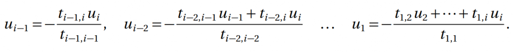
$\left\lbrace\begin{array}{rcl} t_{1,1}x_1+t_{1,2}x_2+\dots +t_{2,n}x_n&=&0\\ t_{2,2}x_2+\dots +t_{1,n}x_n&=&0\\ \vdots\\ t_{n,n}x_n&=&0 \end{array}\right.$

Si tous les coefficients $t_{1,1}$

, … , $t_{n,n}$

sont non nuls, alors en résolvant le système (en partant de la dernière ligne), on trouve $x_n=x_{n-1}=\dots=x_1=0$

. Donc, $\mathrm{Ker}(T)=\big\{(0,\dots,0)\big\}$

. Donc, $T$

est inversible.
Supposons que les coefficients $t_{1,1}$

, … , $t_{n,n}$

ne soient pas tous non nuls. On peut alors considérer le plus petit entier $i$

de $[[1,n]]$

tel que $t_{i,i}=0$

. On pose alors le vecteur $(u_1,\dots,u_n)$

où :

pour tout $j\in [[i+1,n\rrbracket]]$

, $u_{j}=0$

;

$u_i=1$

;

on définit récursivement :

Le vecteur $(u_1,\dots,u_n)$

est non nul et appartient à $\mathrm{Ker}(T)$

. Donc, $T$

n’est pas inversible. On retrouve que $T$

est inversible si, et seulement si, ses coefficients diagonaux sont non nuls.
En transposant, on obtient un résultat similaire pour les matrices triangulaires inférieures.

Théorème

Soit $A\in\mathcal{M}_{n,p}(\mathbb{K})$

. On a :

$p = \mathrm{rg}(A) + \mathrm{dim}(\mathrm{Ker}(A)).$

Démonstration

Soit $f:\mathbb{K}^p\to\mathbb{K}^n$

l’application linéaire canoniquement associée à $A$

. Comme $\mathbb{K}^p$

est de dimension finie, on peut appliquer le théorème du rang à l’application linéaire $f$

$\mathrm{dim}(\mathbb{K}^p)=\mathrm{rg}(f) + \mathrm{dim}(\mathrm{Ker}(f)).$

Or, $\mathrm{dim}(\mathbb{K}^p)=p$

et, par définition $\mathrm{Ker}(f)=\mathrm{Ker}(A)$

, $\mathrm{rg}(f)=\mathrm{rg}(A)$

. Donc,

$p = \mathrm{rg}(A) + \mathrm{dim}(\mathrm{Ker}(A)).$

Proposition

On ne modifie pas le rang d’une matrice en la multipliant à droite ou à gauche par une matrice inversible.

Démonstration

Soient $A\in\mathcal{M}_{n,p}(\mathbb{K})$

et $Q\in\mathrm{GL}_n(\mathbb{K})$

. On considère $f:\mathbb{K}^p\to\mathbb{K}^n$

(respectivement $g:\mathbb{K}^n\to\mathbb{K}^n$

) l’application linéaire canoniquement associée à $A$

(respectivement $Q$

). Par opération, $g\circ f:\mathbb{K}^p\to\mathbb{K}^n$

est l’application linéaire canoniquement associée à $Q A$

. D’où, $\mathrm{Im}(g\circ f) = \mathrm{Im}(Q A).$

De plus, $Q$

est inversible, donc $g$

est un automorphisme. Or, on ne change pas le rang d’une application linéaire en composant à gauche par un isomorphisme. Donc, $\mathrm{rg}(Q A) = \mathrm{rg}(g\circ f) = \mathrm{rg}(f) = \mathrm{rg}(A).$

On traite de la même manière la multiplication à droite par une matrice inversible.

Corollaire

Soient $A\in\mathcal{M}_{n,p}(\mathbb{K})$

, $P\in\mathrm{GL}_p(\mathbb{K})$

et $Q\in\mathrm{GL}_n(\mathbb{K})$

. Alors,

$\mathrm{rg}(A)=\mathrm{rg}(Q A P).$

Démonstration

D’après la proposition précédentes, comme les matrices $P$

et $Q$

sont inversibles :

$\mathrm{rg}(Q A P)=\mathrm{rg}(Q A)=\mathrm{rg}(A).$

Théorème

Soit $A\in\mathcal{M}_n(\mathbb{K})$

S’il existe $B\in \mathcal{M}_n(\mathbb{K})$

tel que $A B= I_n$

, alors $A$

est inversible et $A^{-1}=B$

S’il existe $B\in \mathcal{M}_n(\K)$

tel que $B A= I_n$

, alors $A$

est inversible et $A^{-1}=B$

Démonstration

On suppose qu’il existe $B\in \mathcal{M}_n(\mathbb{K})$

tel que $A B= I_n$

.
On considère $f:\mathbb{K}^n\to\mathbb{K}^n$

(respectivement $g:\mathbb{K}^n\to\mathbb{K}^n$

) l’application linéaire canoniquement associée à $A$

(respectivement $B$

). Par opération, $f\circ g:\mathbb{K}^n\to\mathbb{K}^n$

est l’application linéaire canoniquement associée à $A B$

. Comme $A B=I_n$

, on a $f\circ g=\mathrm{Id}_{\mathbb{K}^n}$

.
Or, $f$

est un endomorphisme et $\mathbb{K}^n$

est de dimension finie. Donc, par théorème $f$

est un automorphisme et $f^{-1}=g$

. Donc, $A$

est inversible et $A^{-1}=B$

.
L’autre cas se traite de la même manière.

Proposition

Soit $(A,B)\in\mathcal{M}_{n,p}(\mathbb{K})\times \mathcal{M}_{p,q}(\mathbb{K})$

. On a :

$\mathrm{rg}(AB)\leq \min\big(\mathrm{rg}(A),\mathrm{rg}(B)\big).$

Démonstration

On considère $f:\mathbb{K}^p\to\mathbb{K}^n$

(respectivement $g:\mathbb{K}^q\to\mathbb{K}^p$

) l’application linéaire canoniquement associée à $A$

(respectivement $B$

). Par opération, $f\circ g:\mathbb{K}^q\to\mathbb{K}^n$

est l’application linéaire canoniquement associée à $A B$

.
Or, en dimension finie, $\mathrm{rg}(f\circ g)\leq \min\big(\mathrm{rg}(f),\mathrm{rg}(g)\big).$

Donc, par définition du rang d’une matrice $\mathrm{rg}(AB)\leq \min\big(\mathrm{rg}(A),\mathrm{rg}(B)\big).$

Pour tout étudiant en quête d’une compréhension plus profonde, un cours particuliers de mathématiques peut éclairer la notion complexe de la matrice d’une application linéaire. 📘

Cet article est extrait de l’ouvrage Maths MPSI-MP2I. Tout-en-un : cours, méthodes, entraînement et corrigés (éditions Vuibert, juin 2021) écrit par E. Thomas, S. Bellec, G. Boutard. ISBN n°9782311408720